We are interested in asking what these static moments are
for systems of nucleons.
In order to answer this question we need to break down the
contribution into parts arising from the orbital
motion of charges (giving a contribution from the velocity
of the proton charge) and a part coming from the
intrinsic spin of the nucleons.
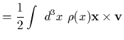
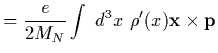
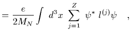
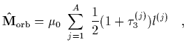
Let us begin by forming the contribution to the magnetic moment
arising from the orbital motion of the proton charge.
The current density of a charge distribution with velocity ![]() is given by
is given by
![]() .
Therefore, our definition of
.
Therefore, our definition of ![]() leads to
leads to
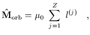
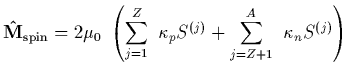
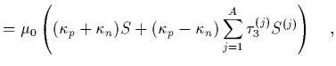
It is easy to include the contribution to the magnetic moment from
the intrinsic magnetic moments of the
neutron and proton.
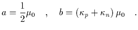
You will recall the the magnetic moment of the proton is
![]() and
magnetic moment of the neutron is
and
magnetic moment of the neutron is
![]() .
Recalling that there is a "g-factor" of 2 for spin
.
Recalling that there is a "g-factor" of 2 for spin
![]() particles we have that
particles we have that
Let me make some comments here. We have made some big assumptions getting
to this point.
Firstly, we have assumed that the only charged currents in the nucleus are
those from the motion of the
nucleons. We have neglected the contributions from mesons, which we know
are present in a field theory
description of nucleons, and as we saw last time are responsible for the
long-range part of the interaction.
Secondly, we have assumed that the nucleons retain their free-space ``identity'',
by which I mean that their
magnetic moments in a nuclear environment are the same as those in free-space.
Corrections to this are a bit harder as we can only ever measure S-matrix
elements and not the individual
contributions.
Clearly, these assumptions will be exact in the limit that the nuclear interactions
``turn-off'', as they then would not ``know'' about each other.
So one might guess that corrections to these results behave like
![]() .
I will leave this subject at this point, to return to later.
This is just a warning, NOT to stop thinking about this!
.
I will leave this subject at this point, to return to later.
This is just a warning, NOT to stop thinking about this!
We will be wanting to form matrix elements of the above operators
between states of good ![]() and
and ![]() ,
and not good
,
and not good ![]() (tensor type interactions).
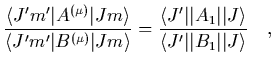
In order to proceed we need to know how to take such matrix elements
and we will need a simple application
of the Wigner-Eckhart theorem, that we will briefly derive.
(tensor type interactions).
In order to proceed we need to know how to take such matrix elements
and we will need a simple application
of the Wigner-Eckhart theorem, that we will briefly derive.
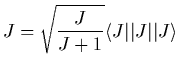
The Wigner-Eckhart theorem tells us that the matrix element of a tensor
operator
![]() of rank
of rank
![]() has matrix elements between states of good total angular momentum
has matrix elements between states of good total angular momentum ![]() of the form
of the form
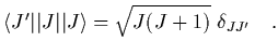
To continue, we note that the matrix element of a scalar operator
formed by contracting the angular momentum
generators with a vector operator ![]() ,
must be proportional to the
reduced matrix element of
,
must be proportional to the
reduced matrix element of ![]() .
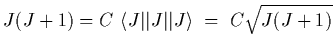
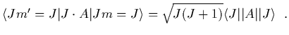
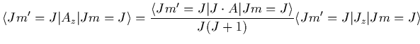
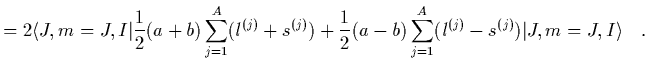
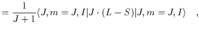
We can then determine the constant of proportionality by setting
.
We can then determine the constant of proportionality by setting
![]() as follows
as follows
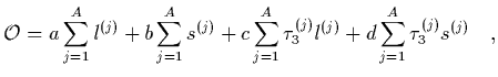
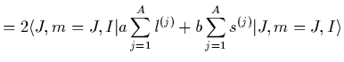
As an application of this result to the magnetic moment, consider an
operator of the form
Applying this relation to the magnetic moments of Mirror nuclei,
e.g. ![]() and
and ![]() ,
where the nuclei only differ by the
nucleon on top of the
,
where the nuclei only differ by the
nucleon on top of the ![]() closed shell
being either a proton or a neutron
(the nuclear wavefunctions are identical except for the
closed shell
being either a proton or a neutron
(the nuclear wavefunctions are identical except for the ![]() quantum
number) ,
quantum
number) ,
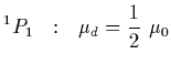
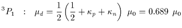
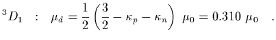
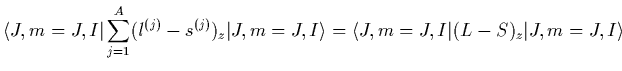
Lets get back to our nucleus of interest for the moment, the deuteron.
We want to find out what we expect
its magnetic moment is for the possible spin-space wavefunctions that
it can possible have.
It is clear from eq. (33) that is magnetic moment is (![]() ,
,
![]() )
)
As we know that the deuteron wavefunction is a linear combination
of ![]() and
and ![]() states,
we realize that the contributions to the magnetic moments will add
incoherently, as they are in a different
partial wave and this, for a mixing angle
states,
we realize that the contributions to the magnetic moments will add
incoherently, as they are in a different
partial wave and this, for a mixing angle ![]() as defined
last time we have that
as defined
last time we have that
Notice that the result is independent of the form of the radial wavefunction. This is the most naive estimate of the D-state admixture, in the most naive single particle model of the nucleus. There are corrections arising from meson exchange, for example, we might imagine attaching a photon to any lines in the graph we drew last time responsible for the potential between nucleons. The graphs we are keeping here are those where the photon attaches to a nucleon, but there are other graphs we have not retained where the photon attaches to the exchanged meson.
![$\displaystyle = 2 \mu_0\ \sum_{j=1}^A\ \left(
{1\over 2}(1+\tau_3^{(j)}) \left[...
...ppa_n\right)
+ {1\over
2}\left(\kappa_p-\kappa_n\right)
\right] S^{(j)}
\right.$](img91.gif)
![$\displaystyle \left. +
{1\over 2}(1-\tau_3^{(j)}) \left[ {1\over 2}\left(\kappa...
...ppa_p\right)
+ {1\over
2}\left(\kappa_n-\kappa_p\right)
\right] S^{(j)} \right)$](img92.gif)

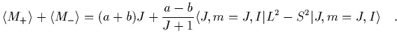
![$\displaystyle \mu_+ + \mu_- = \mu_0\left[
\left({1\over 2}+\kappa_p+\kappa_n\ri...
...r 2}-\kappa_p-\kappa_n\right) {\langle L^2-S^2\rangle\over J+1}
\right]
\ \ \ .$](img134.gif)
![$\displaystyle \mu_d= {\mu_0\over 2} \left[
\left({1\over 2}+\kappa_p+\kappa_n\r...
...er 2}-\kappa_p-\kappa_n\right) {\langle L^2-S^2\rangle\over 2 }
\right]
\ \ \ .$](img138.gif)